Arrival Rate vs Concurrency: Open and Closed Workload Models
Understand open and closed workload models, why slow systems change closed-loop demand, and how to avoid coordinated omission.
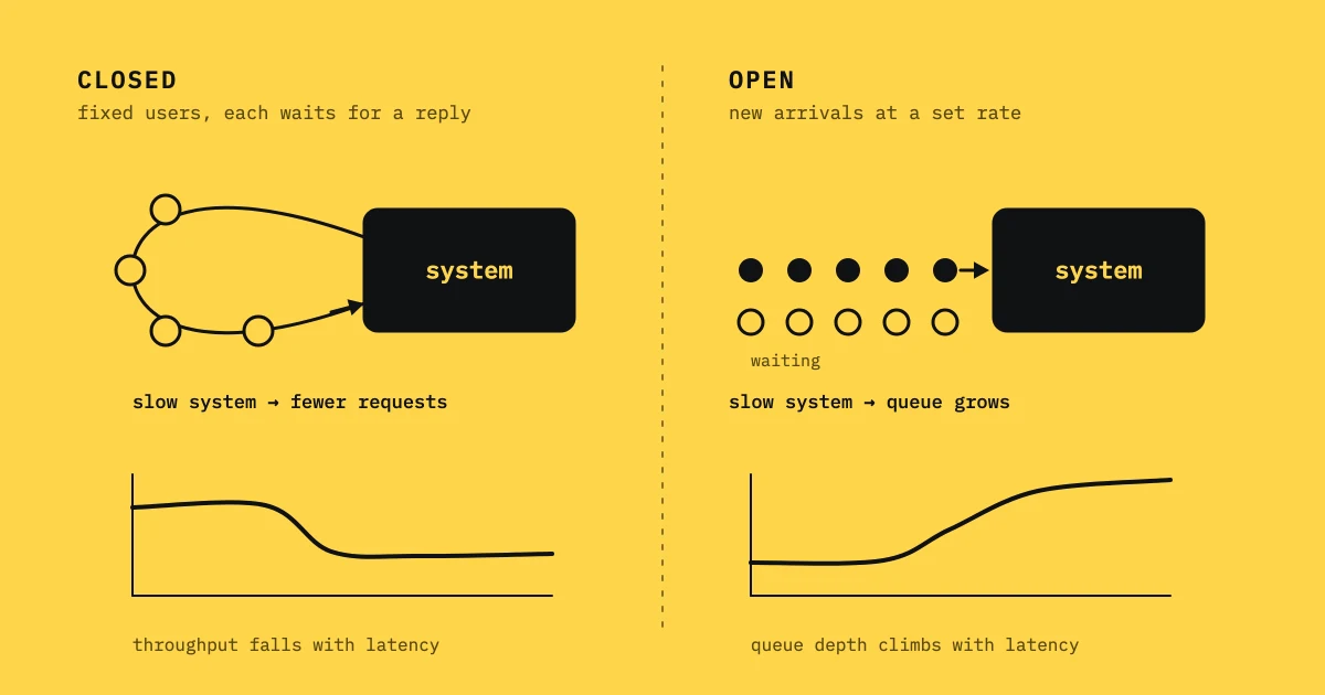
Concurrency and arrival rate are different controls. Concurrency describes work that is active or in flight. Arrival rate describes new work entering over time. The difference matters most when the target slows. A closed model waits with its existing users. An open model keeps sending demand unless backpressure changes it.
Closed models follow actors
In a closed model, a fixed population performs a journey, waits for its response, thinks, and begins again. If the service gets slower, each actor spends longer in the loop and starts fewer iterations. That matches a bounded group of people waiting on a page.
It can also understate queueing pressure from an upstream producer that keeps sending work. A dashboard that reports only VUs can look stable while throughput falls, because every actor is blocked. Keep iteration rate and response time beside the active population.
Open models follow arrivals
An open model schedules new work at a rate independent of whether prior work completed. It resembles incoming requests, messages, webhook deliveries, or users arriving at a public boundary. When service capacity falls below arrivals, in-flight work and queue time grow.
An open model still needs limits. Define maximum backlog, timeout, retry and load-shed behavior. A test that keeps adding work after you know the target is unhealthy has no safety policy. Record scheduled, accepted, completed, rejected, and abandoned work separately.
A simple scenario comparison
Consider a hypothetical endpoint with 100 ms response time. A closed group of 100 users can produce roughly 1,000 iterations per second if there is no think time. If response time rises to 2 seconds, the same population can produce closer to 50 iterations per second. The model cut achieved demand because the users are waiting.
An open scenario scheduled at 1,000 arrivals per second keeps presenting that pressure. The system may queue or reject work, and the test shows whether it does so safely. Neither result is “the real number” until you know which production invariant matters.
Coordinated omission in plain language
If a load generator waits for a slow response before starting the next sample, it does not record the requests that would have arrived during that wait. The measured distribution then leaves out the worst waiting period. This is called coordinated omission.
An open schedule can show more of the omitted demand, but only if the test tool records late starts, queue time, dropped work and client limits. An overloaded generator can create a similar blind spot. Verify achieved arrivals and generator health before interpreting a tail.
Choose with four questions
- Does the source of demand keep producing work when responses slow?
- Is the scarce thing a bounded active population or an independent arrival stream?
- Should overload queue, shed, reject, or retry?
- Which metric proves that the schedule was actually achieved?
Answer these in the test brief. If journeys have different answers, use separate scenarios instead of one compromise model.
Watch the boundaries
Define whether arrival means a browser navigation, a transaction, an API request, or a job. A transaction may contain several requests and retries. Define when it starts and completes. For queues, measure enqueue-to-ack and enqueue-to-finish separately.
Use Little’s Law to sanity-check averages, but do not turn an average relationship into a percentile claim. In an open overload scenario, a growing in-flight count is expected. It is not a reporting bug.
Report both control and outcome
A useful result says: model type, planned rate or population, achieved rate, active work, response distribution, errors, queue time, retries, and generator health. Compare open and closed runs only when the question permits it. Keep their charts labeled so a reader does not mistake one for the other.
The decision is about meaning. Choose arrival rate when demand is independent, concurrency when the actor population is the invariant, and both when the system has layered boundaries. Then make any load-shed and recovery behavior visible in the result.
A boundary-by-boundary example
An API may receive a fixed webhook arrival rate, enqueue work, and expose a status endpoint read by bounded user sessions. Use an open model for webhook arrivals and a closed model for status viewers. Measure enqueue acceptance, queue depth, job completion, and viewer experience separately. A single VU number would erase the independent producer and the waiting users.
When the queue fills, decide whether the producer receives a rejection, a retryable response, or a durable acceptance. Model the client behavior that follows, including backoff and jitter. An open test without a retry policy can create a load pattern no responsible client would send. A closed test without the producer can miss the queue entirely.
Use a timeline, not a single graph
Plot arrivals, active work, queue age, completions, and errors on one time axis. At the first ramp, a closed population may reduce iterations as latency rises. In the open scenario, arrivals remain scheduled while queue age grows. Mark when backpressure activates. The timeline shows how the model behaves and gives operators a safe abort point.
After the run, compare the planned invariant with the observed one. If active users stayed constant but achieved rate fell, the closed model behaved as designed. If scheduled arrivals stayed constant but accepted work fell, inspect load shedding or generator health.
For recovery, reduce arrivals while continuing to observe queue age and completion. A closed population may recover as actors finish, while an open producer may keep the queue above capacity. Test the drain policy separately and state whether it prioritizes oldest work, newest work, or a bounded batch.
Use a simple table to keep the model visible: source of demand, control variable, overload behavior, completion event, and recovery rule. If one journey is a person and another is a queue producer, give them separate rows. The table speeds up design review. It also stops a late script change from quietly turning an arrival schedule into a closed loop.
Validate the schedule under pressure
Before a long run, write down the expected timeline for one actor and one producer. Include start, response, retry, timeout, and completion events. This catches a common mistake: a client-side timeout may start another iteration while the original request is still running. The resulting overlap changes concurrency and can duplicate a write even though the script appears to have one loop.
Instrument the producer and consumer sides separately. For an open workload, record scheduled starts, starts actually emitted, accepted work, rejected work, retries, and completions. For a closed workload, record active actors, iteration starts, response time, think time, and abandoned sessions. Compare these fields over the same windows. A single “requests per second” chart cannot show whether missing work was never emitted, rejected at admission, or is still waiting in a queue.
Use a small saturation trial to verify the interpretation. Increase load until one signal changes, then hold briefly and reduce it. If an open producer keeps its schedule while queue age rises, the target is receiving pressure. If the schedule falls first, inspect worker capacity or a coordinator. If a closed population produces fewer iterations while latency rises, that is expected feedback. It does not show that the target accepted fewer planned arrivals. Mark these transitions on the result.
Finally, keep retry policy and drain behavior in the scenario contract. State whether retries count as new arrivals, whether a rejected job is a failed business outcome, and how long completion is observed after arrivals stop. With these details, model comparisons are reproducible, and a late helper change cannot quietly turn one workload into another.