Little’s Law for Load Testers: Concurrency, Throughput, and Time

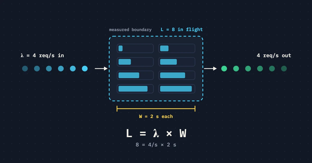
Little’s Law is a small equation with one useful job in a load plan: it catches assumptions that contradict each other. In a stable system, the average number of items in the system equals the average arrival or throughput rate times the average time in the system. For a load tester, that makes it a sanity check on concurrency, work rate, and time. It does not promise capacity.

The equation in plain language

Write it as L = λW: L is the average number of items in the system, λ is the average rate through it, and W is the average time each item spends there. For an API, the items might be in-flight requests. For a queue, they are jobs. For a user journey, they may be active iterations.

Say a hypothetical service completes 4 transactions per second, and each transaction spends 2 seconds inside the measured boundary. The average in-flight count should be about 8. If a plan says the same boundary holds 80 active transactions at 4 per second and 2 seconds, something does not add up. Review the measurement window, the definition of work, or the assumptions.

Where testers use it

Use the equation to estimate a first VU count from observed throughput and response time. Use it to read a growing queue: if the arrival rate stays above the completion rate, L grows. Use it to check whether a reported concurrency number includes think time, client-side waiting, or only server processing.

It also explains why latency eats concurrency in a closed model. If 100 virtual users stay active and each full iteration takes longer, fewer iterations finish per unit of time. The users are still there, but throughput changes. Read open and closed workload models before you treat a VU count as a traffic rate.

Know its assumptions

Little’s Law describes long-run averages for a stable system. It does not need a particular distribution. A short ramp, or a system with a growing queue, may not be in steady state, though. A flash spike, a warm-up period, or a draining queue needs a timeline. One average pasted into the equation will not do.

Define the boundary. If W measures only server time and L counts browser sessions waiting on think time, the units do not match. If throughput counts retries and completions count only successful transactions, the two sides describe different work. State whether redirects, polling, retries, and asynchronous work are included.

Percentiles are not interchangeable

The equation uses averages. User objectives often use p95 or p99. Do not put a p95 into W and call the result an average concurrency. You can use percentile observations to bound scenarios, but label the result as a planning estimate. A heavy tail can push the average time up in a way that intuition built on the median misses.

Put a histogram and a timeline next to the equation. If the average queue time rises while the median holds steady, a slow group of requests may be piling up. If both rise at a ramp step, a shared resource may be saturated. The latency percentiles guide covers the difference.

A worked planning example

Take an order journey with a measured arrival target of 20 completed orders per second and an average measured time of 1.5 seconds across API and queue processing. The rough in-flight count is 20 × 1.5 = 30. Add a separate 5-second wait on the payment provider, and you have to define the boundary. Include the wait and the estimate changes. Exclude it and track that dependency as a separate measurement.

Now say the run schedules 20 arrivals but only achieves 14 because the workers are saturated. Plugging 20 into Little’s Law as throughput would overstate the observed completions. Record the scheduled rate and the achieved rate separately. The gap is itself evidence that the system or the generator cannot sustain the requested workload.

Turn the check into test design

Before the run, calculate the expected concurrency for each journey and scenario. During the run, compare active work, achieved rate, and measured time. Afterward, investigate mismatches. Do not bend the data to fit. A queue that keeps growing is a capacity signal, not an arithmetic error.

Do not make the equation a pass/fail rule on its own. Use explicit latency, error, queue, and completion criteria. Little’s Law tells you whether the numbers are consistent with each other. It does not tell you whether the experience is acceptable.

Keep the workload labels and measurements this check needs. The habit is simple: state the boundary, keep units consistent, show the arithmetic, and label estimates as estimates.

Use it to find a missing queue

Take a worker system with 10 jobs arriving per second and an average completion time of 3 seconds. If it is stable, the measured boundary should hold about 30 jobs. If the queue holds 300 jobs and keeps growing, one of three things is true: completion time is measured too narrowly, arrivals are counted at a different boundary, or the system is not stable. The mismatch tells you where to look.

Repeat the calculation for each stage: accepted by the API, waiting in the queue, executing in a worker, and completed. Do not add those populations together as if they were the same item. One job may pass through several stages. Line up the start and end events before you apply the equation.

During a load run, annotate deploys, autoscaling, cache warm-up, and dependency incidents. Averages that span those transitions can make the equation look wrong when the system was not stationary. Little’s Law stays useful as long as the units and windows stay visible.

Use the check in incident reviews too. If operators report a growing queue while the completion rate and average service time have not changed, check whether arrivals include retries or duplicate deliveries. The arithmetic can expose an instrumentation mismatch before the team changes worker capacity.

Keep units explicit in the report: requests per second, seconds in the boundary, and in-flight requests. For a multi-stage job, report each stage instead of adding counts that do not belong together. When a reviewer can follow the units from the source metric to the conclusion, the equation protects the analysis instead of decorating it.

Use the equation to question a reported result. If 20 jobs per second spend 2 seconds in a worker boundary, about 40 should be in flight. If a dashboard shows 200, ask whether it counts queue wait, retries, or a different stage. Do not “fix” the dashboard until the event definitions agree. The difference may point to the exact backlog you need to test.

For an interactive journey, write down whether time includes think time. Fifty active users who each spend 10 seconds in a measured boundary give about 5 completed iterations per second, but only if the boundary and the cycle are defined the same way. A different pause or retry policy changes the answer. The equation checks the model. It is not a shortcut for picking a virtual user count.

Keep a small worksheet for every conclusion: boundary name, arrival rate, measured residence time, in-flight definition, and the time window used for each. Say a checkout endpoint gets 8 requests per second and each spends 1.5 seconds inside the service. An expected 12 requests in flight is a useful check, but it does not explain a queue outside the service. If the observed count is higher, split active work from queued work and compare the same timestamps. If it is lower, look for sampling, dropped spans, or a rate measured at a different hop. This keeps a correct formula from justifying the wrong scaling action.