Why Average Response Time Lies Under Load

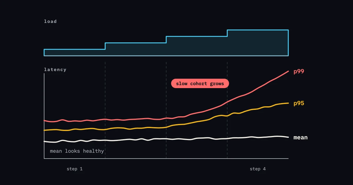
Average response time is easy to read and easy to misuse. It can look healthy while a real group of requests waits behind a queue, retries a dependency or hits a cold path. Under load, treat the average as a starting clue. It does not tell you what users experienced.

How a small tail disappears

Take 99 requests that complete in 100 ms and one that takes 10 seconds. The arithmetic mean is about 199 ms. That number describes no request in the sample. It also makes the slow request look minor, although one user waited one hundred times longer than the common case.

The effect grows when traffic mixes fast cache hits with slow misses, reads with writes, or anonymous requests with authenticated flows. One blended mean can improve because more easy requests arrived while the checkout tail got worse.

Read a distribution, not a headline

Start with counts and a histogram. Look for a single compact peak, a long tail, multiple modes, or a second cluster that appears only after a ramp step. A p50 shows the middle request. A p95 shows how far the slower edge reaches. A p99 shows a still smaller cohort. Always include the sample count and time window.

Percentiles do not explain cause. A p95 that rises from 300 ms to 700 ms is important only in context: which operation, which load, which status, which region, and which response-time boundary? Compare the same labels across runs. Don’t average percentiles from separate workers and call the result the global percentile. Merge raw counts or use a distribution-aware aggregation.

Pair latency with throughput

Latency without achieved throughput can hide a test that barely ran. A generator may report a great p95 because it never reached the requested arrival rate. Record scheduled arrivals, completed operations, dropped work, active users, and retries. If demand is fixed and throughput flattens while latency accelerates, the system may be approaching its useful capacity boundary.

For a closed virtual-user model, slowdown can reduce the number of iterations started. That may be the behavior you want to model, but it can hide queue pressure. Read open and closed workload models and keep the model visible in the report.

Segment before you explain

Break the result down by journey, endpoint, method, status, assertion, payload shape, and dependency where possible. A global p95 can be fine while the one write that matters has a high failure tail. Conversely, a noisy health-check endpoint can make a blended chart look worse than the customer flow.

Separate transport success from business success. An HTTP 200 containing an error object is not a successful checkout. A timeout may be a target failure, a client timeout, or a generator resource issue. Label those categories and use the highest-consequence journey to set the decision.

Connect tails to mechanisms

Tail latency often points to waiting, not raw compute: a connection pool, lock, queue, cache miss, remote call, garbage collection pause or rate limiter. Check target telemetry in the same time window. A request histogram tells you that the tail exists; queue depth and pool wait can explain why.

Do not treat correlation as proof. If database wait and p99 rise together, isolate the hypothesis with a smaller experiment: hold the application load steady, vary the pool or query shape in a safe environment, and see whether the tail responds. Keep the experiment’s assumptions in the result.

Set criteria people can defend

Choose percentile thresholds by consequence and baseline. A checkout might require p95 under an agreed user-facing objective and zero lost writes. A background export may have a completion-time objective instead. Add an error criterion and a generator-validity criterion. Define warm-up, steady-state windows, and sample minimums before the run.

Don’t chase every tail movement. Distributed systems have noise, and a tiny sample makes p99 unstable. Compare distributions over the same workload and environment, then ask whether the effect is large enough to change the release decision. A threshold is a policy your team sets. The endpoint does not come with one.

A practical report layout

Put the decision and workload at the top. Follow with throughput and errors, then latency percentiles and a histogram. Show the slowest labeled journeys and the target signals that support or challenge a mechanism. Keep the average as a small context metric, not the headline.

Close the report by naming the slow cohort, achieved workload, business outcome, and next mechanism to investigate. If any of those are missing, the average is still hiding the evidence the decision needs.

A small numerical sanity check

Take a hypothetical sample of 1,000 requests: 900 complete in 120 ms, 90 in 400 ms, and 10 in 5 seconds. The mean is about 191 ms, while the p99 is near 5 seconds. If the 10 slow requests are checkout writes, a global mean is a poor release signal even though it is mathematically correct. Show the counts and labels so the decision maker can see the cohort.

Now split the same sample by cache state. If the 900 fast requests are warm reads and the 100 slower requests are cold or mutating paths, the next experiment is clear: hold the journey mix and vary cache preparation, then inspect backend calls and pool wait. The segmentation explained the mechanism. The average did not.

Use this kind of example in reviews, but keep hypothetical numbers clearly marked. For real criteria, use the service owner’s objective and a comparable baseline. Averages are still useful for capacity arithmetic and trend context. They mislead when they stand in for the distribution, correctness or the experience of the slow cohort.

The tail is a product question

The average helps when its meaning is explicit. Compare it with the number of completed samples, the operation mix and a set of quantiles for each important journey. If the mean moves while the p95 and p99 stay stable, check the mix and sample weights before you call it a performance change. If the mean is flat while the tail widens, look at the slow cohort right away.

Separate successful responses, timeouts, retries and rejected work in the report. Mixed together, they can make a bad client experience look tidy. Keep the calculation method the same between runs, and write down whether the value is request time, journey time or time spent waiting on a dependency. A reviewer can then reproduce the summary and pick the next experiment, instead of arguing about which single number sounds best.

Ask who experiences the slow requests and what they are doing when they wait. A p99 on a read-only recommendation call may need a different response than a p95 on a payment authorization. A retry may recover a transient read but duplicate a write. Segment the result by consequence before choosing an action.

Use a timeline to join the distribution to system state. Mark ramp steps, deployments, autoscaler events, cache resets, and dependency alerts. If the tail begins after a pool reaches its limit, the next experiment is targeted. If it appears only on one worker, examine the measuring instrument. If no mechanism correlates, report an observation, not a diagnosis.

When presenting the result, put counts beside every summary. “p95 increased” is incomplete without sample size, workload, and operation. A tiny tail movement over a handful of observations should not carry the same weight as a repeated shift over thousands of successful business transactions. The report stays precise without pretending performance is free of noise.

If an average is the only signal you have, say so and avoid a strong conclusion. Add percentile and count instrumentation before you use the result for a release decision. Better evidence often comes from a small labeling change, not a larger test.

When a team must report one number, pair it with the slow-cohort criterion and sample count. The summary stays short, and the mean cannot erase the experience the release decision exists to protect. The summary should lead to the next experiment instead of ending the conversation.

When the distribution changes, keep the slow cohort’s route and dependency context so the next investigation starts from evidence instead of an average.